Wave models

All wave models are implemented in such a way that there is a crest at x=0 at t = 0 and the waves are traveling in the positive x-direction. The origin of the coordinate system is on the sea floor, which is assumed to be horizontal. The default acceleration of gravity is 9.81, so the input quantities should be given in the SI system.

Airy

This is the simplest wave theory, a single cosine wave. It is included mostly for testing the other models and is only valid in the limit of very low waves in very deep water.

Stokes

Stokes waves of 1st to 5th order are implemented following John D. Fenton’s 1985 paper A Fifth‐Order Stokes Theory for Steady Waves. By increasing the requested order N, the code will include more and more expansion coefficients, starting from linear Airy waves at 1st order and properly replicating 2nd, 3rd, 4th and finally 5th order Stokes waves. Any higher order wave requested will issue a warning and return the fift order solution.

Stokes waves are good approximation in the deep water limit. No time consuming calculations are required to generate these waves and the computations will not diverge. Both of these issues can be problematic for stream function waves that need to optimize a non-linear function of many parameters.

Further details and analytical expression for all the coefficients in the perturbation expansion can be found in the original paper, available on John D. Fentons web pages.

Fenton

Fenton stream function wave theory is a high order regular wave theory based on truncated Fourier series approximating the stream function. This method of constructing non-linear regular waves was pioneered by Dean (1965). Our implementation is based on Rienecker and Fenton’s 1981 paper, A Fourier approximation method for steady water waves, which is often refered to as “Fenton” stream function wave theory to differentiate it from the original “Dean” stream function wave theory.

The method is based on collocation (solving the non-linear equations exactly in N + 1 points) and is based on Newton–Raphson iterations to tackle the non-linearities. The unknowns are the expansion coefficients \(B_j\), the wave elevation \(\eta(x_m)\), the stream functions value at the free surface \(Q\) and the Bernoulli constant at the free surface \(R\).

The stream function a-priori satisfies the bottom boundary condition at z=0 and also the Laplace equation \(\nabla^2\Psi=0\). It is defined as

\[\Psi(x, z) = B_0 z + \sum_{j=1}^{N}B_j\frac{\sinh jkz}{\cosh jkD}\cos jkx,\]

which is non-linear in \(\eta\) on the free surface where \(z=\eta\). To find the unknowns the following conditions are requested to be met:

• The free surface is a stream line, such that \(\Psi(x, \eta) = -Q\).

• The pressure is constant at the free surface (Bernoulli constant \(R\)).

• The wave height is \(H\), such that \(\eta(0) - \eta(\lambda/2) = H\)

• The mean wave elevation is \(D\), such that \(\int_0^{\lambda/2} \eta\,\mathrm d x = D \lambda / 2\).

Further details and analytical expression for all terms of the Jacobian matrix used in the Newton-iterations can be found in the original paper, available on John D. Fentons web pages.

Air phase models

Raschii was origially written to provide good initial conditions for an exactly divergence free two-phase Navier-Stokes solver based on DG FEM, Ocellaris. In order to initialise the domain with a divergence free velocity field it is important to also compute the velocities in the air phase in a consistent manner.

ConstantAir

The velocity in the air phase is horizontal with speed equal to the wave phase speed. This is mostly useful when using a blended total field, see Combining the air and wave velocities.

FentonAir

The Fourier series stream function from Rienecker and Fenton (1981) is used also for the air phase. Using a stream function ensures an exactly divergence free velocity field.

The Fenton stream function is linear in the unknown parameters on the free surface when the wave elevation \(\eta\) is known. The air-phase velocities are computed after the water wave has been established, so this means that the expansion coefficients \(B_{1..N}\) can be found by a simple linear solve to satisfy that the free surface is a stream function also in the air phase.

The same collocation method as in the Fenton wave model is used to construct the equation system for the unknown coefficients and the same equi-distant collocation points are used. In order to use the Fenton stream function the z-coordinate is flipped such that the air velocities are purely horizontal a specified “depth” above the free surface.

Combining the air and wave velocities

The combined velocity field in the water and air domains can be obtained by simply changing the stream function at the free surface. The result obtained by using Fenton stream functions in both the water and air phases can be seen in the below figure. The velocities normal to the surface are continuous as one would expect since the free surface is a stream line in both domains. The velocities parallel to the surface are discontinuous with magnitues of approximately the same size, but different directions. This is similar to what can be found in many textbooks for potential flow linear waves on the interface between two fluids. Full continuity cannot be enforced without any viscosity. The divergence of the velocity in the resulting field is naturally quite high at the discontinuity when the combined water and air velocity field is projected into a finite element space.

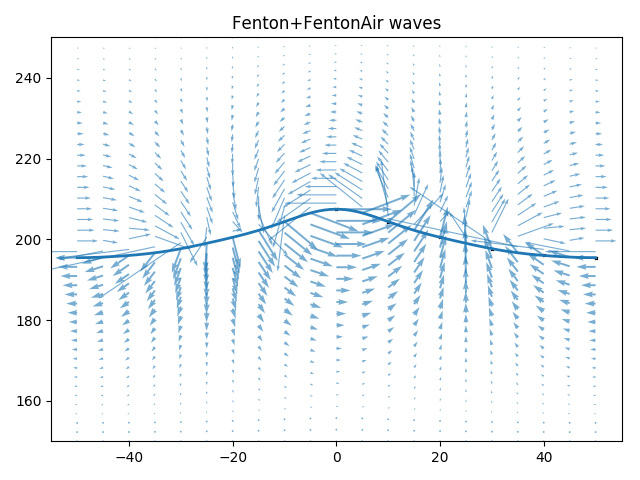
Unblended stream function velocities near the free surface. Fenton wave and FentonAir solution for wave height 12m, depth 200 m and wave length 100 m with an fifth order stream function and a 100 m air layer thickness above the still water height. Produced by python3 demos/plot_wave.py Fenton+FentonAir 12 200 100 -N 5 -a 100 -b 0 -v --ymin 150 --ymax 250.

To combat these problems the two stream functions are blended together. The stream function in the water domain is left entirely undisturbed, but from the free surface up to z = d = air.blending_height + wave.depth the stream function in the water is smoothly transitioned into the the stream function in the air. The blending height can be set to a different value than the height of the air layer—by default it is the same as twice the wave height. The results can be seen in the figure below. The resulting velocity field is exactly divergence free since the blending is done to create a new stream function from which the velocities are calculated.

\[ \begin{align}\begin{aligned}\Psi &= [1 - f(Z)] \Psi_{w}(x,z) + f(Z) \Psi_{a}(x,z),\\Z &= \frac{z - \eta(x)}{d - \eta(x)}\,,\\\mathbf{u}_x &= (1 - f) \frac{\partial\Psi_{w}}{\partial z} + f \frac{\partial\Psi_{a}}{\partial z} - \frac{d f}{d z}\Psi_{w}(x,z) + \frac{d f}{d z}\Psi_{a}(x,z),\\\mathbf{u}_z &= -(1 - f) \frac{\partial\Psi_{w}}{\partial x} - f \frac{\partial\Psi_{a}}{\partial x} + \frac{d f}{d x}\Psi_{w}(x,z) - \frac{d f}{d x}\Psi_{a}(x,z),\end{aligned}\end{align} \]

where the blending function \(f(Z)\) is a constant equal to 0.0 in the water (\(\Psi=\Psi_w\) for \(z <\eta(x)\)) and 1.0 above the air blending zone (\(\Psi=\Psi_a\) for \(z > d\)). Raschii uses a fifth order smooth step function for \(f(Z)\) in the blending zone. This function has zero first and second derivatives at the top and bottom of the blending zone.

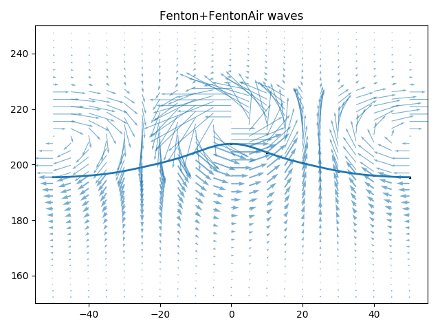
Blended stream function velocities near the free surface. Fenton wave and FentonAir solution for wave height 12m, depth 200 m and wave length 100 m with an fifth order stream function and a 100 m air layer thickness above the still water height. Produced by python3 demos/plot_wave.py Fenton+FentonAir 12 200 100 -N 5 -a 100 -b 30 -v --ymin 150 --ymax 250.